Representations of Sound: Time and Frequency Domains
Background:
When a computer records digital audio, it measures the sound pressure level multiple times per second. These measurements are often called samples. Being digital, the samples are quantized -- that is, they can only take on certain discrete values as compared to the continuous range of possible values in the actual analog sound wave. Commonly, the samples can take on the integer values between -32768 and +32767 (the range of numbers representable with 16 bits) with positive values representing the sound pressure level being above the ambient atmospheric pressure and negative values representing the sound pressure level being below the ambient atmospheric pressure.
The samples are recorded many times per second. A common sampling rate is 44,100 samples per second. The Nyquist-Shannon sampling theorem tells us that we need to sample at twice the highest frequency that we want to reproduce. Thus, sampling at 44,100 Hz allows the digital audio to reproduce frequencies up to 22,050 Hz which is about 10% above the highest frequency that humans typically hear.
We could plot the samples on a graph. The X axis would represent time and the Y axis the sound pressure level (the value of the sample). In the graph below, the distance between adjacent peaks represents 100 samples with a sampling rate of 44,100 Hz. Thus, the sound has a fundamental frequency of 441 Hz (44,100 / 100 = 441). Listening to it would sound like the A above middle C which has a fundamental frequency of 440 Hz.
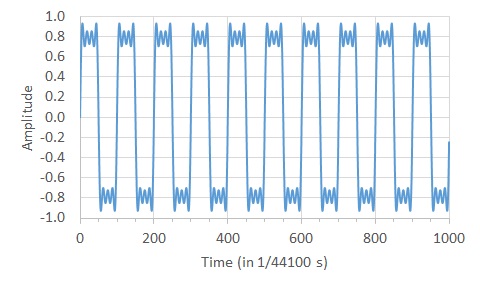
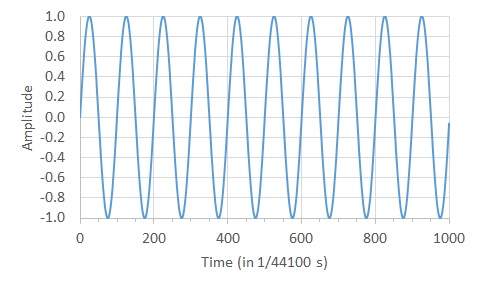
The sound wave shown above looks somewhat like a square wave. If you compare it to a 441 Hz pure tone (shown below), it is obvious that it is not a pure sinusoid and not a pure tone.
That demonstrates a problem with looking at the samples of the sound wave. Psychologically, the pitch of the sound (correlated with its frequency) is important. In this example, it is easy to determine that there is a 441 Hz sound in the wave, but it isn't easy to determine what other frequencies are in it -- and there are other frequencies in it, otherwise it would be a pure sinusoid. What we would like to know is what are the frequencies in the sound.
Fortunately there is a mathematical procedure that can tell us which frequencies are present in the sound wave. That procedure is call the Fourier transform and is named after its founder Jean-Baptiste Joseph Fourier. The mathematics behind the Fourier transform are beyond the scope of this page (Google it if you want to know more), but what it does is very useful to us. The Fourier transform translates a set of data in the time domain into the frequency domain and vice versa. What does that mean? It means that it can be used to take the samples (which were sampled across time -- they are in the time domain) and determine the sinusoids (frequency and amplitude -- the frequency domain) that could be used to create the samples. This is called a Fourier analysis. The Fourier transform can also do the opposite -- take the sinusoids and recreate the samples. This is called Fourier synthesis.
If you do a Fourier analysis on the samples shown in the first graph, you get results that look like this:
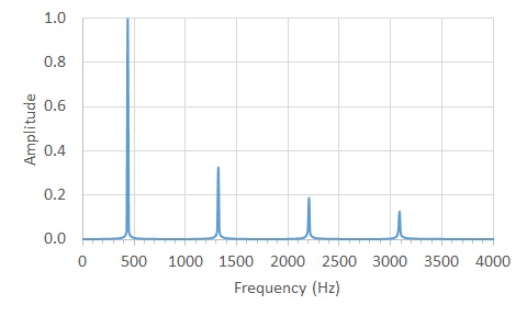
Looking at the results of the Fourier analysis tells us that there are four frequencies present in the sound wave:
| Frequency | Amplitude |
| 441 Hz | 1 |
| 1323 Hz = 3 X 441 Hz | 1/3 |
| 2205 Hz = 5 * 441 Hz | 1/5 |
| 3087 Hz = 7 * 441 Hz | 1/7 |
Fourier analysis and synthesis form the basis of digital signal processing and allows us to do things like speed up the rate of a recording without changing the pitch. To double the rate (say play a 60 second recording in 30 seconds), use a Fourier analysis to determine the frequencies, divide each frequency by two (which would half the pitch) and use a Fourier synthesis to get the samples. Replace the first and second samples with a single value -- their average. Repeat for the third and fourth samples, for the fifth and sixth samples, and every other pair of samples. When played, the samples come twice as fast because there are only half as many, so the pitch is doubled. Doubling the half pitch restores the original pitch.
Since the pitch of a voice is correlated with the interpretation of such things as the dominance of the speaker (see Puts, Hodges, Cárdenas & Gaulin, 2007)), you could use Fourier analysis and synthesis to artificially lower the pitch of your voice and become the most dominant person in the world! (Oh, wait, that is an overgeneralization....)
The Activity:
This activity allows you to load a sound file and see a representation of it in both the time and frequency domains. The duration of the sound should be fairly short -- no more than a second or two. Only sounds files of the type .WAV can be loaded. If you don't have any .WAV files handy, you can download one of these by right clicking on the link and then selecting save. The loaded files do not leave your computer -- all processing occurs locally. If you hear something inappropriate, it is because it was already on your computer.
When you load a sound, it will play. Always practice safe listening habits. Always start with the volume at a low level and gradually increase the volume until it is at a comfortable level. If you are using earbuds, if someone else can hear the sound then it is at too high of a level and you must decrease the volume. Listening to overly loud sounds (even for a very short period of time if the sound is sufficiently loud) can lead to permanent hearing loss. Most speakers / earbuds / headphones can produce sounds loud enough to cause permanent hearing loss.
Some sounds that you can download, and then load:
The sound wave used in the graphs in the background section.
Me saying the word "perception"
One purr from my buddy
Once you have a short .WAV file on your computer, you can load it by first clicking on the "Choose File" button. Select the file. Then click on the "Graph It" button.
Below each graph is a slider control which will control the window of data shown in the graph above the control. For example, initially, the frequency domain graph shows the amplitudes of the frequencies between 0 and 500 Hz. Slowly sliding the frequency window slider to the right will show the amplitudes for other windows of frequencies -- e.g. between 250 and 750 Hz.
Toward the bottom is a media control. Clicking on its play button will play the sound.
Select a .WAV file:
Frequency window: 0 Hz: 19,500 Hz
Sample / Time window: Sample 0: Sample
Play the sound:
Frequency Domain Data: (checking this will slow things down)
Sample (Time Domain) Data: (checking this will slow things down a lot)