Using SPSS for One Way Analysis of Variance
![]()
This tutorial will show you how to use SPSS version 12 to perform a one-way, between- subjects analysis of variance and related post-hoc tests.
This tutorial assumes that you have:
The one way analysis of variance (ANOVA) is an inferential statistical test that allows you to test if any of several means are different from each other. It assumes that the dependent variable has an interval or ratio scale, but it is often also used with ordinally scaled data.
In this example, we will test if the response to the question "If you could not be a
psychology major, which of these majors would you choose? (Math, English, Visual Arts, or
History)" influences the person's GPAs. We will follow
the standard steps for performing hypothesis tests:
SPSS assumes that the independent variable (technically a quasi-independent variable in this case) is represented numerically. In the sample data set, MAJOR is a string. So we must first convert MAJOR from a string variable to a numerical variable. See the tutorial on transforming a variable to learn how to do this. We need to automatically recode the MAJOR variable into a variable called MAJORNUM.
Once you have recoded the independent variable, you are ready to perform the ANOVA. Click
on Analyze | Compare Means | One-Way ANOVA:
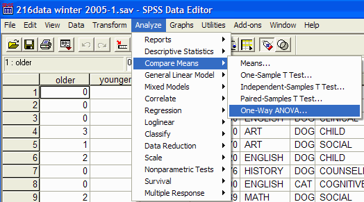
The One-Way ANOVA dialog box appears:

In the list at the left, click on the variable that corresponds to your dependent
variable (the one that was measured.) Move it into the Dependent List by clicking on the
upper arrow button. In this example, the GPA is the variable that we recorded, so we click
on it and the upper arrow button:
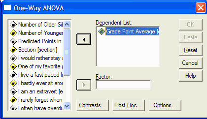
Now select the (quasi) independent variable from the list at the left and click on it.
Move it into the Factor box by clicking on the lower arrow button. In this example, the
quasi-independent variable is the recoded variable from above, MAJORNUM:

Click on the Post Hoc button to specify the type of multiple comparison that you
would like to perform. The Post Hoc dialog box appears:
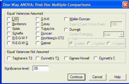
Consult your statistics text book to decide which post-hoc test is appropriate for you.
In this example, I will use a conservative post-hoc test, the Tukey test. Click in the
check box next to Tukey (not Tukey's-b):
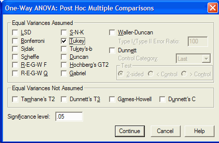
Click on the Continue Button to return to the One-Way ANOVA dialog box. Click on the
Options button in the One-Way ANOVA dialog box. The One-Way ANOVA Options dialog box
appears:
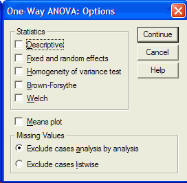
Click in the check box to the left of Descriptives (to get descriptive statistics),
Homogeneity of Variance (to get a test of the assumption of homogeneity of variance) and
Means plot (to get a graph of the means of the conditions.):
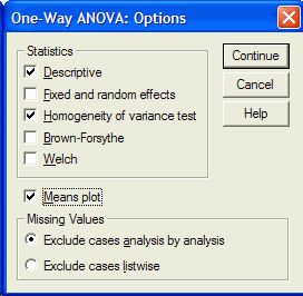
Click on the Continue button to return to the One-Way ANOVA dialog box. In the One
Way ANOVA dialog box, click on the OK button to perform the analysis of variance. The
SPSS output window will appear. The output consists of six major sections. First, the
descriptive section appears:

For each dependent variable (e.g. GPA), the descriptives output gives the sample size,
mean, standard deviation, minimum, maximum, standard error, and confidence interval for
each level of the (quasi) independent variable. In this example, there were 7 people
who responded that they would be a math major if they could not be a psychology major, and their mean
GPA was 3.144, with a standard deviation of 0.496. There were 16 people who would be
an English major if they could not be a psychology major, and their mean GPA was
2.937 with a standard deviation of 0.5788.

The Test of Homogeneity of Variances output tests H0:
σ2Math = σ2English =
σ2Art =
σ2History.
This is an important assumption made by the analysis of variance. To interpret this output,
look at the column labeled Sig. This is the p value. If the p value is less than or equal
to your α level for this test, then you can reject
the H0 that the variances are equal. If the p value is greater than
α level for this test, then we fail to reject H0
which increases our confidence that the variances are equal and the homogeneity
of variance assumption has been met. The p value is .402. Because the
p value is greater than the α level, we
fail to reject H0 implying that there is little evidence that the variances are not equal and the homogeneity of
variance assumption may be reasonably satisfied.

The ANOVA output gives us the analysis of variance summary table. There are six
columns in the output:
| Column | Description |
|---|---|
| Unlabeled (Source of variance) | The first column describes each row of the ANOVA summary table. It tells us that the first row corresponds to the between-groups estimate of variance (the estimate that measures the effect and error). The between-groups estimate of variance forms the numerator of the F ratio. The second row corresponds to the within-groups estimate of variaince (the estimate of error). The within-groups estimate of variance forms the denominator of the F ratio. The final row describes the total variability in the data. |
| Sum of Squares | The Sum of squares column gives the sum of squares for each of the estimates of variance. The sum of squares corresponds to the numerator of the variance ratio. |
| df | The third column gives the degrees of freedom for each estimate of
variance. The degrees of freedom for the between-groups estimate of variance is given by the number of levels of the IV - 1. In this example there are four levels of the quasi-IV, so there are 4 - 1 = 3 degrees of freedom for the between-groups estimate of variance. The degrees of freedom for the within-groups estimate of variance is calculated by subtracting one from the number of people in each condition / category and summing across the conditions / categories. In this example, there are 2 people in the Math category, so that category has 7 - 1 = 6 degrees of freedom. There are 16 people in the English category, so that category has 16 - 1 = 15 degrees of freedom. For art, there are 15 - 1 = 14 degrees of freedom. For history there are 7 - 1 = 6 degrees of freedom. Summing the dfs together, we find there are 6 + 15 + 14 + 6 = 41 degrees of freedom for the within-groups estimate of variance. The final row gives the total degrees of freedom which is given by the total number of scores - 1. There are 45 scores, so there are 44 total degrees of freedom. |
| Mean Square | The fourth column gives the estimates of variance (the
mean squares.) Each mean square is calculated by dividing the sum of square by its
degrees of freedom. MSBetween-groups = SSBetween-groups / dfBetween-groups MSWithin-groups = SSWithin-groups / dfWithin-groups |
| F | The fifth column gives the F ratio. It is calculated by dividing
mean square between-groups by mean square within-groups. F = MSBetween-groups / MSWithin-groups |
| Sig. | The final column gives the significance of the F ratio. This is the p value. If the p value is less than or equal your α level, then you can reject H0 that all the means are equal. In this example, the p value is .511 which is greater than the α level, so we fail to reject H0. That is, there is insufficient evidence to claim that some of the means may be different from each other. |
We would write the F ratio as: The one-way, between-subjects analysis of variance failed to reveal a reliable effect of other major on GPA, F(3, 41) = 0.781, p = .511, MSerror = 0.292, α = .05.
The 3 is the between-groups degrees of freedom, 41 is the within-groups degrees of
freedom, 0.781 is the F ratio from the F column, .511 is the value in the Sig. column
(the p value), and 0.292 is the within-groups mean square estimate of variance.
When the F ratio is statistically significant, we need to look at the
multiple comparisons output. Even though our F ratio is not statistically
significant, we will look at the multiple comparisons to see how they are
interpreted.
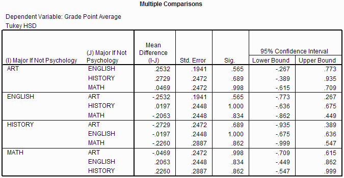
The Multiple Comparisons output gives the results of the Post-Hoc tests that you requested. In this example, I requested Tukey multiple comparisons, so the output reflects that choice. Different people have different opinions about when to look at the multiple comparisons output. One of the leading opinions is that the multiple comparison output is only meaningful if the overall F ratio is statistically significant. In this example, it is not statistically significant, so technically I should not check the multiple comparisons output.
The output includes a separate row for each level of the independent variable. In
this example, there are four rows corresponding to the four levels of the quasi-IV. Lets
consider the first row, the one with major equal to art. There are three sub-rows
within in this row. Each sub-row corresponds to one of the other levels of the quasi-IV.
Thus, there are three comparisons described in this row:
| Comparison | H0 | H1 |
|---|---|---|
| Art vs English | H0: µArt = µ English | H1: µArt ≠ µEnglish |
| Art vs History | H0: µArt = µ History | H1: µArt ≠ µHistory |
| Art vs Math | H0: µArt = µ Math | H1: µArt ≠ µMath |
The second column in the output gives the difference between the means. In this example, the difference
between the GPA of the people who would be art majors and those who would be
English majors is 0.2532. The third column gives the standard
error of the mean. The fourth column is the p value for the multiple comparison. In this
example, the p value for comparing the GPAs of people who would be art majors with those
those who would be English majors is 0.565, meaning that it is unlikely that these means are different
(as you would expect given that the difference (0.2532) is small.) If the p values is
less than or equal to the α level, then you can
reject the corresponding H0. In this example, the p value is .565 which is
larger than the α level of .05, so we fail to
reject H0 that the mean GPA of the people who would be art majors is different from the mean
GPA of the people who would be English majors. The final two columns give you the 95% confidence interval.
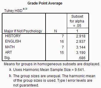
The next part of the SPSS output (shown above) summarizes the results of the multiple comparisons procedure. Often there are several subset columns in this section of the output. The means listed in each subset column are not statistically reliably different from each other. In this example, all four means are listed in a single subset column, so none of the means are reliably different from any of the other means. That is not to say that the means are not different from each other, but only that we failed to observe a difference between any of the means. This is consistent with the fact that we failed to reject the null hypothesis of the ANOVA.
The final part of the SPSS output is a graph showing the dependent variable (GPA) on the
Y axis and the (quasi) independent variable (other major) on the X axis:
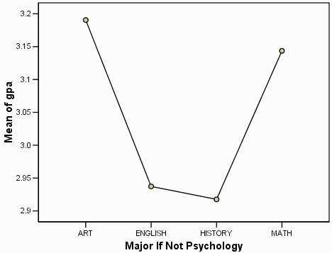
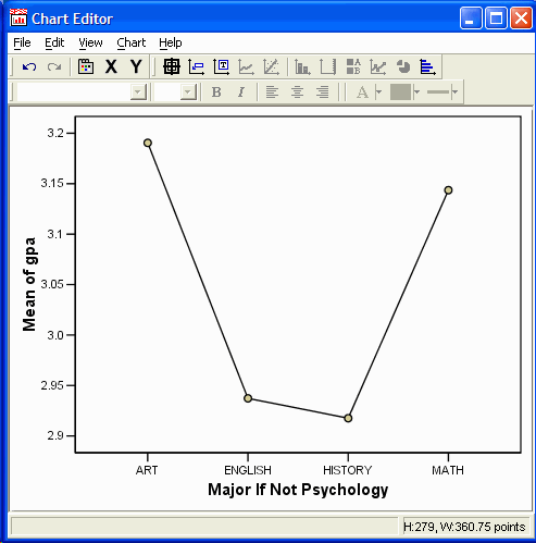
Because the quasi-independent variable is nominally scaled, the plot really should be
a bar plot. Double click on the plot to invoke the SPSS Chart Editor:
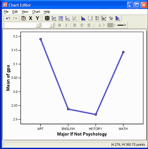
In the Chart Editor, click on one of the data points:
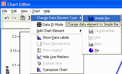
In the Chart Editor, select
Chart | Change Data Element Type | Simple Bar:
The new bar graph appears in
the editor:
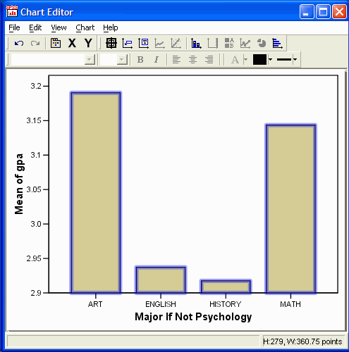
Make any other changes to the bar graph that you want. (See the tutorial on editing graphs if you don't remember how to make changes.)
Close the Chart Editor by selecting File | Close in the chart editor.