Using SPSS for Factorial, Between-Subjects Analysis of Variance

Using SPSS for Two-Way, Between-Subjects ANOVA

This tutorial will show you how to use SPSS version 12.0 to perform a two factor, between- subjects analysis of variance and related post-hoc tests.

This tutorial assumes that you have started SPSS (click on Start | All Programs | SPSS for Windows | SPSS 12.0 for Windows).

The factorial analysis of variance (ANOVA) is an inferential statistical test that allows you to test if each of several independent variables have an effect on the dependent variable (called the main effects). It also allows you to determine if the main effects are independent of each other (i.e., it allows you to determine if two more independent variables interact with each other.) It assumes that the dependent variable has an interval or ratio scale, but it is often also used with ordinally scaled data.

In this example, we will look at the results of an actual quasi-experiment. In the study, people were randomly assigned either to come to class all the time, or to never come to class and to get the lecture notes from the World Wide Web. Those who came to class are in the Lecture condition, while those who did not come to class are in the Distance Learning condition. The students were also divided according to their GPA prior to the class. There were people with Higher GPAs and people with Lower GPAs. Thus, this is a 2 X 2 between-subjects, factorial design. One of the dependent variables was the total number of points they received in the class (out of 400 possible points.) The following table summarizes the data:

Class GPA Points in Class

Distance High 332.00

Distance High 380.00

Distance High 371.00

Distance High 366.00

Distance High 354.00

Distance Low 259.50

Distance Low 302.50

Distance Low 296.00

Distance Low 349.00

Distance Low 309.00

Lecture High 354.67

Lecture High 353.50

Lecture High 304.00

Lecture High 365.00

Lecture High 339.00

Lecture Low 306.00

Lecture Low 339.00

Lecture Low 353.00

Lecture Low 351.00

Lecture Low 333.00

Class	GPA	Points in Class
Distance	High	332.00
Distance	High	380.00
Distance	High	371.00
Distance	High	366.00
Distance	High	354.00
Distance	Low	259.50
Distance	Low	302.50
Distance	Low	296.00
Distance	Low	349.00
Distance	Low	309.00
Lecture	High	354.67
Lecture	High	353.50
Lecture	High	304.00
Lecture	High	365.00
Lecture	High	339.00
Lecture	Low	306.00
Lecture	Low	339.00
Lecture	Low	353.00
Lecture	Low	351.00
Lecture	Low	333.00

A more compact way of presenting the same data is:

Class

Distance Lecture

GPA Low 259.50
302.50
296.00
349.00
309.00 306.00
339.00
353.00
351.00
333.00

High 332.00
380.00
371.00
366.00
354.00 354.67
353.50
304.00
365.00
339.00

	Class
Distance	Lecture
GPA	Low	259.50 302.50 296.00 349.00 309.00	306.00 339.00 353.00 351.00 333.00
High	332.00 380.00 371.00 366.00 354.00	354.67 353.50 304.00 365.00 339.00

The columns define the level of the first factor, while the rows define the level of the second factor.

The first step is to enter the data into SPSS. You will have to create three variables:

Variable Name Type Variable Label Value Labels Measurement

Class Numeric Class Condition 1 = Distance
2 = Lecture Nominal

GPA Numeric High or Low GPA 1 = High GPA
2 = Low GPA Ordinal

Points Numeric Number of Points in Class Scale (interval or ratio)

Variable Name	Type	Variable Label	Value Labels	Measurement
Class	Numeric	Class Condition	1 = Distance 2 = Lecture	Nominal
GPA	Numeric	High or Low GPA	1 = High GPA 2 = Low GPA	Ordinal
Points	Numeric	Number of Points in Class		Scale (interval or ratio)

(If you don't remember how to create variables, see the tutorial on defining variables.)

Now that the data have been defined, you need to enter the data into SPSS. Remember that each row represents an individual and each column represents a variable. For example, you would enter a "1" into the first column and first row because the first observation in the data table above is in the Distance condition and the Distance condition is represented by a "1". Press the right arrow key to move to the next column and enter a "1" again. This time the "1" stands for a person with a High GPA. Press the right arrow key again, and enter "332.00" (or just 332 since that is the same value) because the first observation earned 332 points in the class. Press the down arrow key once and the left arrow key twice to move to the first column of the second row. Enter the remaining data in a similar fashion.

Carefully go back through your data to make sure that you have entered it correctly. Have your neighbor check your work. Errors at this stage can have major impacts on the analyses. It is often helpful to turn on the view value labels options (View | Value Labels):

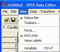
This replaces the "1"s and "2"s that you entered with their corresponding labels (e.g. "1" is replaced with "Distance".)

We will be performing three statistical tests at once in this example -- one for each of the two possible main effects and one for the possible interaction effect:

Write the null and alternative hypotheses:

Main Effect of Type of Class	Main Effect of GPA	Interaction Effect of Type of Class and GPA
H₀: µ_Distance = µ_Lecture H₁: not H₀ This hypothesis asks if the mean number of points received in the class is different for the distance condition and the lecture condition.	H₀: µ_{High GPA} = µ_{Low GPA} H₁: not H₀ This hypothesis asks if the mean number of points received in the class is different for people with high GPAs and people with low GPAs.	H₀: µ_{Distance, High GPA} - µ_{Distance, Low GPA} = µ_{Lecture, High GPA} - µ_{Lecture, Low GPA} H₁: not H₀ This hypothesis asks if the effect of high versus low GPA is the same for people in the distance condition as it is for people in the lecture condition.

Where µ represents the mean number of points received in the class.

Specify the α level: α = .05
Determine the statistical test to perform: In this case, the number of points received in the class is ratio scaled, and we have multiple (2) (quasi) IVs with different people in each condition. The between-subjects, factorial ANOVA is appropriate.

Calculate the appropriate statistic:

SPSS assumes that the independent variables are represented numerically. This is true for this data set. If it was not true, we would have to convert the independent variables from a string variable to a numerical variable. See the tutorial on transforming a variable to learn how to do this.

Once the independent variables are numeric, you are ready to perform the ANOVA. Click on Analyze | General Linear Model | Univariate:

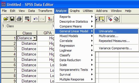
The Univariate dialog box appears:

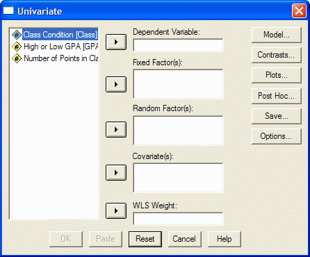
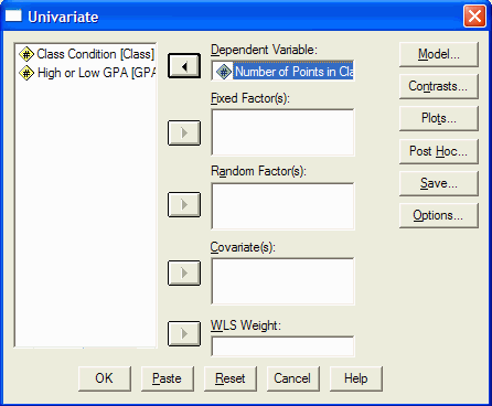
In the list at the left, click on the variable that corresponds to your dependent variable (the one that was measured.) Move it into the Dependent Variable box by clicking on the upper arrow button. In this example, the Number of Points in the Class variable is the dependent variable, so we click on it and the upper arrow button:

Now select one of the independent variables from the list at the left and click on it. Move it into the Fixed Factor(s) box by clicking on the second from top arrow button. Click on the other (quasi) independent variable and move it into the Fixed Factor(s) box by clicking on the second from top arrow button. In this example, the independent variable is the class condition (distance vs lecture) and the quasi-independent variable is whether the person has a high or low GPA. Thus, for each (quasi) independent variable we would click on it and then on the second from top arrow button. The dialog box should now look like this:

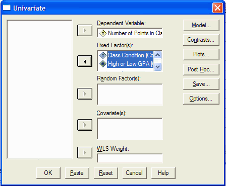
(The difference between Fixed Factor(s) and Random Factor(s) is whether the levels of the (quasi) IVs were randomly selected from all the possible levels of the IV (the random factors) or were all the levels that we are interested in represented in the IV (the fixed factors.) Most undergraduate statistics text books only present the Fixed Factors model.)

Click on the Plots button to specify the type of graphs that you want SPSS to prepare. The Univariate: Profile Plots dialog box appears:

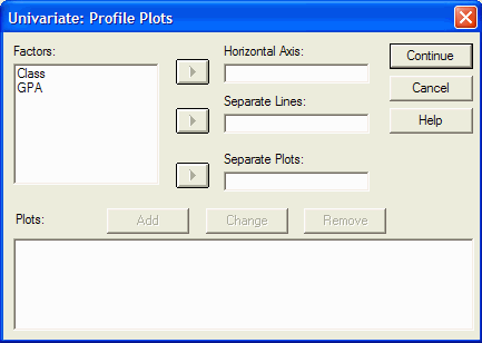
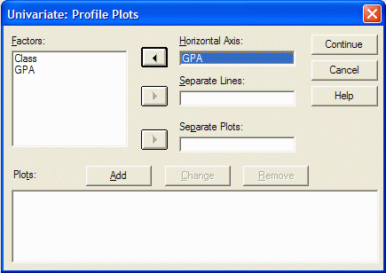
The (quasi) IVs are listed in the Factors box. Select, by clicking on it, the (quasi) IV that you would like to be plotted on the X axis (the horizontal axis). Move it into the Horizontal Axis box by clicking on the upper arrow button. In this example, I am going to plot the GPA variable on the horizontal axis, so I click on it in the Factors list and then click on the upper arrow button:

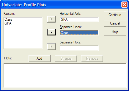
Next, select the (quasi) IV that you want represented as separate lines on the graph. In this example, I want one line for the Distance condition and another line for the Lecture condition, so I will move the Class variable into the Separate Lines box by first clicking on the variable, and then clicking on the middle arrow button:

Now click on the Add button:

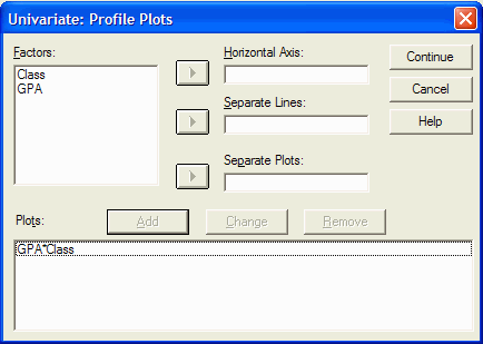
You can specify as many plots as you want by repeating the process. When you are done specifying the plots, click on the Continue button to return to the Univariate dialog box.

If at least one of your (quasi) independent variables has at least three levels, you will want to click on the Post-Hoc button so you can specify which type of multiple comparisons to perform. Even though all of the (quasi) independent variables in this example have only two levels, and therefore we should not perform the multiple comparisons, this is what happens when you click the Post Hoc button:

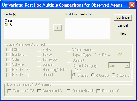
For each independent variables that you want post-hoc tests performed, click on the variable in the Factor(s) list and move it into the Post-Hoc Tests For list by clicking on the arrow button. Then you can specify the type(s) of multiple comparisons, such as Tukey, that you want performed for each variable. When done, click on the Continue button. Because our independent variables each have only two levels, we will not specify any post-hoc tests. (If you do request multiple comparisons for independent variables with only two levels, SPSS will simply ignore your request and issue a warning when the ANOVA is performed.)

From the Univariate dialog box, click on the Options button. The Univariate: Options dialog box appears:

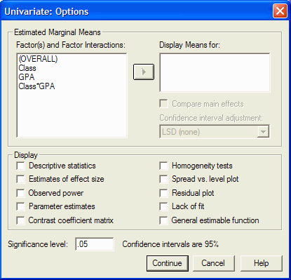
This dialog box allows you to view descriptive statistics for each main effect and / or interaction. Usually you will want means for each main effect and interaction that is listed in the Factor(s) and Factor Interactions list. For each item in the list, click on it and then the arrow button to move that item into the Display Means for box. (If you want to be really fancy, click on the top item in the list, then hold down the shift key and click on the bottom item in the list. All the items should be highlighted. Now click on the arrow button to move them all into the Display Means for list):

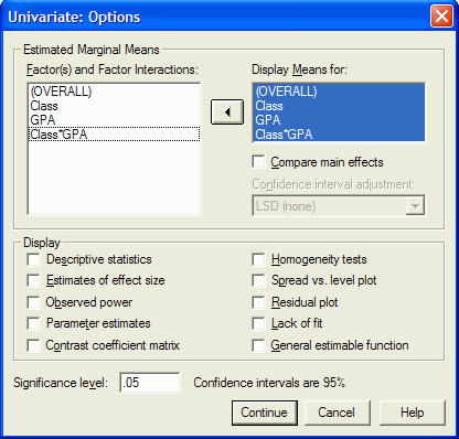
If desired, you can also request that several additional types of statistics be performed. Sometimes it is helpful to have a more complete set of descriptive statistics than just the means. You can get these by clicking in the box to the left of Descriptive Statistics. You can also request SPSS to perform Levene's homogeneity of variance test by clicking in the box to the left of that option:

You can get a description of the option by right clicking on an option. Once you have selected all the desired options, click on the Continue button to return to the Univariate dialog box. In that dialog box, click on OK to actually perform the requested statistics.

Depending on the options that you selected, the output may contain the following (or other) sections:

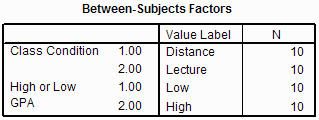
The above section of the output contains a list of the between-subjects independent variables in your ANOVA. It states that there are two between-subjects IVs: Class Condition and High or Low GPA. It also shows that each of the IVs has two levels and the number of observations in each level of each IV. For example, the Class Condition has two levels: 1 -- Distance with 10 observations and 2 -- Lecture with 10 observations.

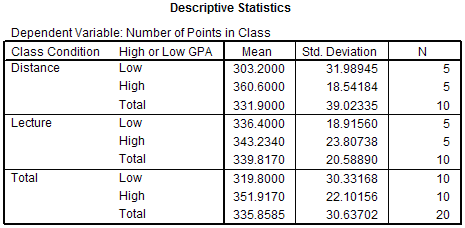
The Descriptive Statistics section of the output gives the mean, standard deviation, and sample size for each condition in the study and the marginal means. In this example, the mean number of points received in the class for the distance learners with a high GPA is 360.6 points. The mean number of points received for the lecture, low GPA people is 336.4 points. The marginal means are given in the rows labeled Total. The mean number of points received for all people in the Distance condition (ignoring whether their GPA is high or low) is 331.9 points. Similarly, the mean number of points received for all people in the high GPA condition (ignoring whether they were in the distance or lecture condition) was 351.917 points.

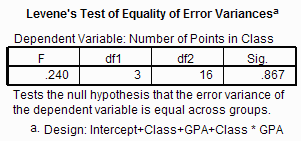
The Levene's Test of Equality of Error Variances section of the output tests one of the assumptions of ANOVA -- namely that the variances of each condition are approximately equal. As in the two-sample t-test and one-way ANOVA outputs, we look at the p value given in the Sig. (significance) column. If that p value is less than or equal to the α level for the test, then you can reject the H₀ that the variances are equal. (Remember, that because we are trying to accept H₀ that the variances are equal, we usually set the α level much higher that we normally would, say to .25.) In this example, the p value (.867) is larger than the α level (.25), so we fail to reject H₀, and basicly assume that H₀ is probably true. That is, it is probably the case that the variances in the groups are approximately equal. (Note: I just accepted the null hypothesis, which normally is not a good thing to do.)

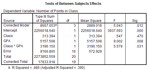
The Tests of Between-Subjects Effecs output gives us the analysis of variance summary table. As in the one-way ANOVA summary table, there are six columns in the output:

Column Description

Source The first column describes each row of the ANOVA summary table. In this example there are four rows that we are primarily interested in:

The row labeled with one of the IVs, e.g. CLASS. This corresponds to the between-groups estimate of variance for the main effect of that IV.
The row labeled with the other IV, e.g. GPA. This corresponds to the between-groups estimate of variance for the main effect of that IV.
The row labeled with both IVs, separated by a *, e.g. CLASS * GPA. This corresponds to the between-groups estimate of variance of the interaction effect of the two IVs.
The row labeled Error. This corresponds to the within-groups estimate of variance.

Type III Sum of Squares The Sum of squares column gives the sum of squares for each of the estimates of variance. The sum of squares corresponds to the numerator of the variance ratio.

df The third column gives the degrees of freedom for each estimate of variance.
The degrees of freedom for the between-groups estimate of variance is given by the number of levels of the IV - 1. In this example there are two levels of the Class IV, so there are 2 - 1 = 1 degrees of freedom for the between-groups estimate of variance for the main effect of Class.

There also are two levels to the GPA variable, so there are 2 - 1 = 1 degrees of freedom of freedom for the between-groups estimate of variance for the main effect of GPA.

The interaction degrees of freedom is given by the product of the main effect degrees of freedom. Thus the interaction effect has 1 X 1 = 1 degrees of freedom associated with its between-groups estimate of variance.

The degrees of freedom for the within-groups estimate of variance is calculated by subtracting one from the number of people in each condition / category and summing across the conditions / categories. In this example, there are 5 people in the Distance, High GPA category, so that category has 5 - 1 = 4 degrees of freedom. There are 5 people in the Distance, Low GPA category, so that category has 5 - 1 = 4 degrees of freedom. For Lecture, High GPA there are 5 - 1 = 4 degrees of freedom. And, for Lecture, Low GPA there also are 5 - 1 = 4 degrees of freedom. Summing the dfs together, we find there are 4 + 4 + 4 + 4 = 16 degrees of freedom for the within-groups estimate of variance.
The final row gives the (corrected) total degrees of freedom which is given by the total number of scores - 1. There are 20 scores, so there are 19 total degrees of freedom.

Mean Square The fourth column gives the estimates of variance (the mean squares.) Each mean square is calculated by dividing the sum of square by its degrees of freedom.
MS_Class = SS_Class / df_Class

MS_GPA = SS_GPA / df_GPA

MS_{Class * GPA} = SS_{Class * GPA} / df_{Class * GPA}

MS_Error = SS_Error / df_Error

F The fifth column gives the F ratios. They are calculated by dividing the appropriate mean square between-groups by mean square within-groups.
F_Class = MS_Class / MS_Error

F_GPA = MS_GPA / MS_Error

F_{Class * GPA} = MS_{Class * GPA} / MS_Error

Sig. The final column gives the significance of the F ratios. These are the p values. If a p value is less than or equal your α level, then you can reject H₀. In this example, there are three p values -- one for each of the two main effects and one for the interaction effect of the two IVs. The p value for the main effect of Class is .470. Since this p value is not less than or equal to the α level, so we fail to reject H₀. That is, there is insufficient evidence to claim that there is a difference between the Distance and Lecture conditions.

Column	Description
Source	The first column describes each row of the ANOVA summary table. In this example there are four rows that we are primarily interested in: The row labeled with one of the IVs, e.g. CLASS. This corresponds to the between-groups estimate of variance for the main effect of that IV. The row labeled with the other IV, e.g. GPA. This corresponds to the between-groups estimate of variance for the main effect of that IV. The row labeled with both IVs, separated by a , e.g. CLASS GPA. This corresponds to the between-groups estimate of variance of the interaction effect of the two IVs. The row labeled Error. This corresponds to the within-groups estimate of variance.
Type III Sum of Squares	The Sum of squares column gives the sum of squares for each of the estimates of variance. The sum of squares corresponds to the numerator of the variance ratio.
df	The third column gives the degrees of freedom for each estimate of variance. The degrees of freedom for the between-groups estimate of variance is given by the number of levels of the IV - 1. In this example there are two levels of the Class IV, so there are 2 - 1 = 1 degrees of freedom for the between-groups estimate of variance for the main effect of Class. There also are two levels to the GPA variable, so there are 2 - 1 = 1 degrees of freedom of freedom for the between-groups estimate of variance for the main effect of GPA. The interaction degrees of freedom is given by the product of the main effect degrees of freedom. Thus the interaction effect has 1 X 1 = 1 degrees of freedom associated with its between-groups estimate of variance. The degrees of freedom for the within-groups estimate of variance is calculated by subtracting one from the number of people in each condition / category and summing across the conditions / categories. In this example, there are 5 people in the Distance, High GPA category, so that category has 5 - 1 = 4 degrees of freedom. There are 5 people in the Distance, Low GPA category, so that category has 5 - 1 = 4 degrees of freedom. For Lecture, High GPA there are 5 - 1 = 4 degrees of freedom. And, for Lecture, Low GPA there also are 5 - 1 = 4 degrees of freedom. Summing the dfs together, we find there are 4 + 4 + 4 + 4 = 16 degrees of freedom for the within-groups estimate of variance. The final row gives the (corrected) total degrees of freedom which is given by the total number of scores - 1. There are 20 scores, so there are 19 total degrees of freedom.
Mean Square	The fourth column gives the estimates of variance (the mean squares.) Each mean square is calculated by dividing the sum of square by its degrees of freedom. MS_Class = SS_Class / df_Class MS_GPA = SS_GPA / df_GPA MS_{Class * GPA} = SS_{Class * GPA} / df_{Class * GPA} MS_Error = SS_Error / df_Error
F	The fifth column gives the F ratios. They are calculated by dividing the appropriate mean square between-groups by mean square within-groups. F_Class = MS_Class / MS_Error F_GPA = MS_GPA / MS_Error F_{Class * GPA} = MS_{Class * GPA} / MS_Error
Sig.	The final column gives the significance of the F ratios. These are the p values. If a p value is less than or equal your α level, then you can reject H₀. In this example, there are three p values -- one for each of the two main effects and one for the interaction effect of the two IVs. The p value for the main effect of Class is .470. Since this p value is not less than or equal to the α level, so we fail to reject H₀. That is, there is insufficient evidence to claim that there is a difference between the Distance and Lecture conditions.

Decide whether to reject H₀ or not. We had three hypotheses, so we must reject or fail to reject each of the three H₀s:

Main Effect of Type of Class	Main Effect of GPA	Interaction Effect of Type of Class and GPA
H₀: µ_Distance = µ_Lecture H₁: not H₀ This hypothesis asks if the mean number of points received in the class is different for the distance condition and the lecture condition. Find the row in the ANOVA summary table that is labeled with this IV (e.g. the row labeled CLASS.) Find the column labeled Sig. The p value at the intersection of the row and column is used to decide whether to reject H₀ or not. If the p value is less than or equal to α, then you can reject H₀. In this example the p value equals .470, which is greater than .05 (α) so we fail to reject H₀. That is, there is insufficient evidence to conclude that the Distance and Lecture means are different. We would write this F ratio as: The 2 X 2 between-subjects analysis of variance (ANOVA) failed to reveal a main effect of class, F(1, 16) = 0.547, MS_e = 572.93, p = .470, α = .05. The 1 is the between-groups degrees of freedom from the row labeled with the IV (CLASS). The 16 is the within-groups degrees of freedom from the row labeled Error. The 0.547 is the F value from the row labeled with the IV (CLASS). MS_e is the mean square error (MS) from the row labeled Error. The .470 is the p value (Sig.) from the row labeled with the IV (CLASS).	H₀: µ_{High GPA} = µ_{Low GPA} H₁: not H₀ This hypothesis asks if the mean number of points received in the class is different for people with high GPAs and people with low GPAs. Find the row in the ANOVA summary table that is labeled with this IV (e.g. the row labeled GPA.) Find the column labeled Sig. The p value at the intersection of the row and column is used to decide whether to reject H₀ or not. If the p value is less than or equal to α, then you can reject H₀. In this example the p value equals .008, which is less than or equal to .05 (α) so we reject H₀. That is, there is sufficient evidence to conclude that the High and Low GPA means are probably different. We would write this F ratio as: The ANOVA revealed a main effect of GPA, F(1, 16) = 9.002, p = .008. The 1 is the between-groups degrees of freedom from the row labeled with the IV (GPA). The 16 is the within-groups degrees of freedom from the row labeled Error. The 9.002 is the F value from the row labeled with the IV (GPA). Notice that we did not fully describe the type of ANOVA performed (e.g. "2 X 2 between-subjects" is missing) and we did not include MS_e or α. These are only included with the first F value that is reported, unless they change as can be true in within- subjects designs.	H₀: µ_{Distance, High GPA} - µ_{Distance, Low GPA} = µ_{Lecture, High GPA} - µ_{Lecture, Low GPA} H₁: not H₀ This hypothesis asks if the effect of high versus low GPA is the same for people in the distance condition as it is for people in the lecture condition. Find the row in the ANOVA summary table that is labeled with both IVs (e.g. the row labeled CLASS * GPA.) Find the column labeled Sig. The p value at the intersection of the row and column is used to decide whether to reject H₀ or not. If the p value is less than or equal to α, then you can reject H₀. In this example the p value equals .031 which is less than or equal to .05 (α) so we reject H₀. That is, there is sufficient evidence to conclude that the effect of having a High versus Low GPA is probably different for Distance and Lecture conditions. We would write this F ratio as: The ANOVA revealed an interaction of class and GPA, F(1, 16) = 5.579, p = .031. The 1 is the between-groups degrees of freedom from the row labeled with both IVs (CLASS * GPA). The 16 is the within-groups degrees of freedom from the row labeled Error. The 5.579 is the F value from the row labeled with both IVs (CLASS * GPA).

The next several sections of the output give various means associated with the data. These means are often reported in the text of a manuscript, or as a table or figure.

The Grand Mean gives the overall mean of all the data.

The Class Condition section gives the marginal means for the levels of the Class IV. That is, it gives the mean of all the data in each level of the IV while ignoring the existence of all other IVs. This information is often presented in the results section of an APA style paper when discussing the main effect of the IV. In this example, the mean number of points received for everyone in the Distance condition is 331.9 points and the mean number of points received for everyone in the Lecture condition is 339.817 points.

The High or Low GPA section is similar to the Class Condition section, except that it deals with the other independent variable. It gives the means of all the data in each level of the GPA variable while ignoring the existence of the other IVs (e.g. CLASS.) As above, this information is often presented in the results section when discussing the main effect of the IV. In this example the mean number of points received for everyone in the High GPA condition is 351.917 points and the mean number of points received for everyone in the Low GPA condition is 319.8 points.

The Class Condition * High or Low GPA section of the output gives the means for each of the conditions in this 2 X 2 between-subjects design. For example, the mean number of points received for people in the Distance, High GPA condition is 360.6 points and the mean number of points received for people in the Lecture, Low GPA condition is 336.4 points.

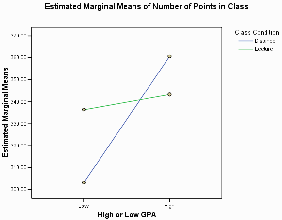
The final part of the SPSS output is a graph showing the dependent variable (Number of Points in the Class) on the Y axis, one of the independent variables (GPA) on the X axis and the other independent variable (CLASS) as separate lines on the graph. You can double click on the graph to edit it, as always.