Using SPSS for Ordinally Scaled Data:
Mann-Whitney U, Sign Test, and Wilcoxon Tests

This tutorial will show you how to use SPSS version 9.0 to perform Mann Whitney U tests, Sign tests and Wilcoxon matched-pairs signed-rank tests on ordinally scaled data.

This tutorial assumes that you have:

• Downloaded the standard class data set (click on the link and save the data file)
• Started SPSS (click on Start | Programs | SPSS 9.0 for Windows)
• Loaded the standard data set

Mann Whitney U Test

The Mann Whitney U test is a non-parametric test that is useful for determining if the mean of two groups are different from each other. It requires that four conditions be met:

1. The dependent variable must be as least ordinally scaled.
2. The independent variable has only two levels.
3. A between-subjects design is used.
4. The subjects are not matched across conditions.

The Mann Whitney U test is often used when the assumptions of the t-test have been violated. Thus it is useful if:

• The dependent variable is ordinally scaled instead of interval or ratio.
• The assumption of normality has been violated in a t-test (especially if the sample size is small.)
• The assumption of homogeneity of variance has been violated in a t-test

In this example, we will determine if people who intend to get a Ph.D. or Psy.D. in psychology are more likely to rely on a calendar or day-planner to remember what they are supposed to be doing (i.e., are people who might become professors more absent minded than other people?)

SPSS assumes that the variable that specifies the category is numeric. In the sample data set, the PhD variable corresponds to the question described above, but it is a string variable. So we will have to recode the variable before we can perform the Mann-Whitney U test. If you don't remember how to automatically recode a variable, see the tutorial on transforming variables. I automatically recoded the PhD variable into a variable called PhDNUM.

As always, we will perform the basic steps in hypothesis testing:

1. Write the hypotheses:
   H₀: µ_PhD µ_{No PhD}
   H₁: µ_PhD < µ_{No PhD}
   Note how the question on the questionnaire is worded. People who respond with a low number (1 = strongly agree) rely on a calendar more than people who respond with a higher number. Thus the hypotheses are "reversed" from what one might think.
2. Determine if the hypotheses are one- or two-tailed. These hypotheses are one-tailed as the null is written with a greater than or equal to sign.
3. Specify the level: = .05
4. Perform the Mann Whitney U test.
   

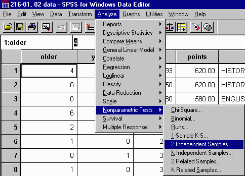
   Select Analyze | Nonparametric Tests | 2 Independent Samples:
   
   

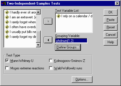
   The Two-Independent-Samples Tests dialog box appears:
   
   

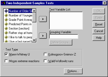
   Select the dependent variable of interest from the list at the left by clicking on it, and then move it into the Test Variable List by clicking on the upper arrow button. In this example, I selected the variable PLANNER and moved it into the Test Variable List box:
   
   

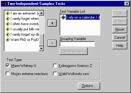
   Select the independent variable of interest from the list at the left by clicking on it, and then move it into the Grouping Variable box by clicking on the lower arrow button. In this example, I selected the variable I automatically recoded earlier (PhDNUM) and moved it into the Grouping Variable box:
   
   

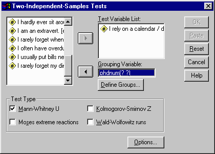
   Next, we must define the groups of the independent variable. Click on the Define Groups button that is just below the Grouping Variable box. The Two Independent Samples: Define Groups dialog box appears:
   
   

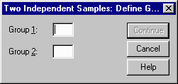
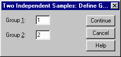
   Enter the value that corresponds to one level of the independent variable in the Group 1 box and the value that corresponds to the other level of the independent variable in the Group 2 box. Since we automatically recoded the PhD variable into the PhDNUM variable, the people who responded No to the question have a value of 1 and the people who responded Yes to the question have a value of 2 (see the SPSS output of the automatic recode operation.) Thus we should enter 1 for group 1 and 2 for group 2:
   
   

   Click on the Continue button in the Two Independent Samples: Define Groups dialog box. The Two-Independent Samples Test dialog box should be on top now. Make sure that the Mann-Whitney U option is selected in the Test Type frame. That is, there should be a check mark next in the box to the left of Mann-Whitney U:
   
   

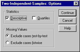
   Click on the Options button. The Two-Independent-Samples: Options dialog box appears:
   
   

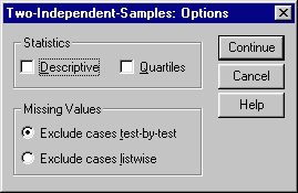
   Select the Descriptive statistics option by clicking in the box to the left of Descriptives if it does not already have a check mark in it:
   
   

   Click on the Continue button in the Two-Independent-Samples: Options dialog box. Click on OK in the Two-Independent-Samples Tests box to perform the Mann-Whitney U test. The SPSS output viewer will appear. It should contain three sections:
   
   

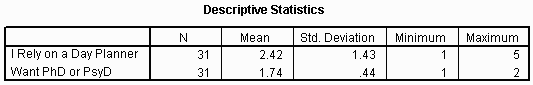
   The first section gives the descriptive statistics for the dependent variable and (less usefully) for the independent variable. In this example, there were 31 people (N) who responded to the PLANNER question. They gave a mean response of 2.42 (between AGREE and UNDECIDED) with a standard deviation of 1.43 (although this number may not be meaningful in this example as standard deviation is not a valid statistic for an ordinally scaled variable.)
   

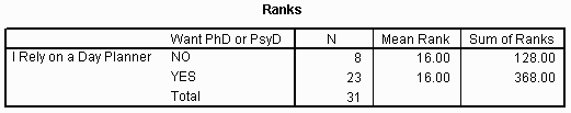
   The second section of the output shows the number (N) of people in each condition (8 people do not intend to get a Ph.D. or Psy.D in psychology and 23 people do) and the mean rank and sum of ranks for each group (useful if you were calculating the U statistic by hand.)
   
   

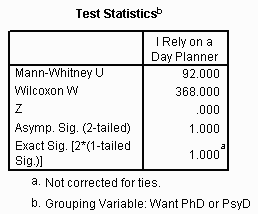
   The final section of the output gives the values of the Mann-Whitney U test (and several other tests as well.) The observed Mann-Whitney U value is given at the intersection of the row labeled Mann-Whitney U and the column labeled with the dependent variable (I rely on a day-planner.) In this example, the Mann-Whitney U value is 92.0. There are two p values given -- one on the row labeled Asymp. Sig (2-Tailed) and the other on the row labeled Exact Sig. [2*(1- tailed Sig.)]. Typically, we will use the Exact significance, although if the sample size is large, the asymptotic signifance value can be used to gain a little statistical power.

5. Decide whether to reject H₀. We will use the exact p value. It is a two-tailed p value, but we have a one-tailed test. So we need to divide the two-tailed p value by 2 to get the one-tailed p value: 1.000 / 2 = .500. Since the exact p value is greater than the specified level (.05), we fail to reject H₀. Thus, we have insufficient evidence to conclude that people who intend to get a Ph.D. or Psy.D. in psychology are more likely to use a day planner or calendar than the people who do not intend to get a Ph.D. or Psy.D. in psychology.

Sign Test and Wilcoxon Matched-Pairs Signed-Rank Test

Both the sign test and the Wilcoxon matched-pairs signed-rank tests are nonparametric statistic that can be used with ordinally (or above) scaled dependent variable when the independent variable has two levels and the participants have been matched or the samples are correlated. Thus, both are useful when a t-test cannot be employed because its assumptions have been violated.

The sign test uses only directional information while the Wilcoxon test uses both direction and magnitude information. Thus the Wilcoxon test is more powerful statistically than the sign test. However, the Wilcoxon test assumes that the difference between pairs of scores is ordinally scaled, and this assumption is difficult to test.

In this example, we will use a fictional data set that is available from here. In this data set, people were matched on their GPA prior to being assigned to one of two conditions: either they were allowed to use an on-line quiz program or they were not allowed to use it. At the end of the semester, the students rated how much they liked the class on a 7-point Likert scale with 1 being that they did not like the class at all and 7 being that they liked the class very much. Notice how the data have been entered into SPSS. There are two variables -- one for the liking score for the people who had the on-line quiz and one for the liking score for the people who did not have the on-line quiz. The data points in each row are matched. That is the two people who gave us scores in the first row have similar GPAs. The two people who gave us scores in the second row have similar GPAs and so on.

We will determine if the mean liking rating is different for the two groups of students.

As always, we will perform the basic steps in hypothesis testing:

1. Write the hypotheses:
   H₀: µ_Quiz = µ_{No Quiz}
   H₁: µ_Quiz µ_{No Quiz}
   
2. Determine if the hypotheses are one- or two-tailed. These hypotheses are two-tailed as the null is written with an equal sign.
3. Specify the level: = .05
4. Perform the sign test and / or Wilcoxon matched-pairs signed-rank test.
   

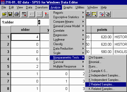
   Select Analyze | Nonparametric Tests | 2 Related Samples:
   
   

   The Two-Related-Samples Tests dialog box appears:
   
   

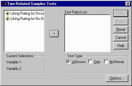
   Select the dependent variable that corresponds to one of the means in the hypothesis from the list at the left by clicking on it. Select the other dependent variable that corresponds to the other mean in the hypothesis from the list at the left by clicking on it as well. You should have two variables highlighted. In this example, the first variable (Liking Rating for On-Line Quiz) corresponds to the first mean in the hypothesis, so I clicked on it. The second variable (Liking Rating for No On-Line Quiz) corresponds to the second mean in the hypothesis, so I clicked on it as well:
   
   

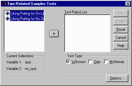
   Move the selected pair of variables into the Test Pair(s) List box by clicking on the arrow button:
   
   

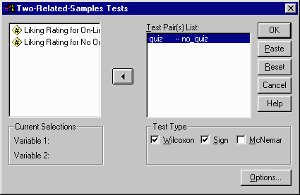
   Select the type of statistical test that you want to perform in the Test Type section of the dialog box. I will select to perform both the Sign test and the Wilcoxon test:
   
   

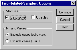
   Click on the Options button. The Two-Related-Samples: Options dialog box appears:
   
   

   Select the Descriptive statistics option by clicking in the box to the left of Descriptives if it does not already have a check mark in it:
   
   

   Click on the Continue button in the Two-Related-Samples: Options dialog box. Click on OK in the Two-Related-Samples Tests box to perform the Sign and Wilcoxon tests. The SPSS output viewer will appear. It should contain five sections:
   
   

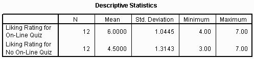
   The first section gives the descriptive statistics for the dependent variable for each level of the independent variable. In this example, there were 12 people (N) in each condition. The On-Line quiz people gave a mean liking rating of 6.000 with a standard deviation of 1.0445 (although this number may not be meaningful in this example as standard deviation is not a valid statistic for an ordinally scaled variable.) The No On-Line quiz people gave a mean liking rating of 4.500 with a standard deviation of 1.3143.
   
   

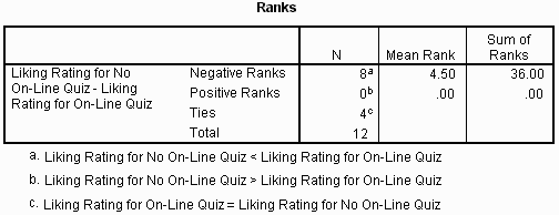
   The second section of the output shows the ranks for the Wilcoxon test. It gives the number of observations (N), 8, in which the No On-Line Quiz people liked the class less than their matched counterpart (The Negative Ranks row). It also gives the number of observations, 0, in which the No On-Line Quiz people liked the class more than their matched counterparts (the Positive Ranks row.) Finally, it gives the number of observations, 4, in which the No On-Line Quiz people liked the class the same amount as their matched counterparts in the On-Line Quiz group (the Ties row.)
   
   

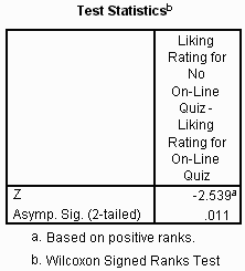
   The third section of the output gives the values of the Wilcoxon test. The p value associated with the Wilcoxon test is given at the intersection of the row labeled Asymp. Sig. (2-tailed) (asymptotic significance, 2-tailed) and the column labeled with the difference of the variables that correspond to the means in the hypothesis (e.g. Liking Rating for No On-Line Quiz - Liking Rating for On-Line Quiz. In this example, the p value for the Wilcoxon test is .011.
   
   

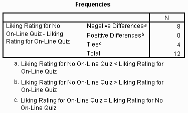
   This section of the output is similar to the ranks section. It is produced for the sign test, while the ranks section is produced for the Wilcoxon test. It gives the number of observations (N), 8, in which the No On-Line Quiz people liked the class less than their matched counterpart (the Negative Differences row). It also gives the number of observations, 0, in which the No On-Line Quiz people liked the class more than their matched counterparts (the Positive Differences row). Finally, it gives the number of observations, 4, in which the No On-Line Quiz people liked the class the same amount as their matched counterparts in the On-Line Quiz group (the Ties row.)
   
   

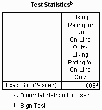
   The final section of the output gives the values of the Sign test. The p value associated with the sign test is given at the intersection of the row labeled Exact Sig. (2-tailed) and the column labeled with the difference of the variables that correspond to the means in the hypothesis (e.g. Liking Rating for No On-Line Quiz - Liking Rating for On-Line Quiz.) In this example, the p value for the sign test is .008.
   

5. Decide whether to reject H₀. If the p value is less than the specified level (.05), we can reject H₀. For the Wilcoxon matched-pairs signed-rank test, the p value was .011 which is less than . Thus we can reject H₀ that the mean liking ratings are the same for the people who had the on-line quiz program available and those who did not. For the sign test, the p value was .008 which is less than . Again, we can reject H₀ that the mean liking ratings are the same for the people who had the on-line quiz program available and those who did not.